
From governing equations to a explainable real time intelligence.
A companion piece to Why generic and black box AI fails on positive displacement pumps, which argued that these machines defeat conventional analytics because the variable governing the failure is not the variable being measured. This article sets out the alternative: how a physics AI engine is composed, trained, verified and bounded before it is allowed to prescribe anything.
1. Two incumbents, each with its own limitations
Fault diagnosis in rotating equipment has been served by two traditions.
The first is model-based, what the industry generally calls white box. It encodes expert knowledge in one of two forms: dynamic models derived from physical conservation laws, or statistical indicators extracted by signal processing. Strictly, only the first is white box in the full sense, since every term is written down and every parameter carries physical units and a physical meaning. Both share the defining characteristic, which is that nothing is learned from the machine. Everything is specified in advance by design and engineering teams.
The consequence is that it is transparent, it extrapolates honestly, and it fails in a specific way: it is rigid. A model written for one machine, one fluid and one duty does not move to the next installation without an engineer rewriting it. Scaling is linear in headcount, worse the analysis output does not keep up with the in-the-now requirement of the operations and maintenance teams.
Rigidity is also a quantitative problem. A recent study of gear pump leakage compared a model using nominal design clearances against measured performance and found an average prediction error of 9.43 percent, with the model consistently overestimating volumetric efficiency and the overestimation growing as pressure rises1. Incorporating the measured wear distribution after running-in reduced that error. A first-principles model with design-sheet parameters is not a description of the pump on your skid. It is a description of a pump that existed briefly, on a test bed, before it was commissioned.
The second tradition is data-driven, the black box, and the inversion of the first: nothing is specified in advance and everything is learned from the machine data. Its limits on this class of machine are set out separately: labels that do not exist at the required density, decisions that are implicit rather than inspectable, and degradation under conditions the training set never contained. The virtual flow metering literature in oil and gas, which has run this comparison at commercial scale for two decades, reaches the same verdict. Data-driven meters post better headline accuracy, but their generalization ability and robustness remain insufficient for wide commercial deployment. Published figures illustrate the gap between benchmark and field: one well-cited series of data-driven virtual meters reported errors of 1.5 percent on gas, 4.2 percent on oil and 4.7 percent on water, while a commercial hybrid product reported 4 percent on multiphase rates over two months for a single well, without reporting robustness across other wells2.
Neither of these limitations is a defect of intelligence. Each tradition is missing what the other has. Physics knows the structure and not the specific machine. Data knows the specific machine and not the structure.
The relevant result from the same literature is that the combination beats both. The metering field calls this grey box, and reports that hybrid approaches outperform pure first-principles models wherever simulated and measured rates diverge, and can reach higher accuracy than machine learning alone.
That is the case for physics AI, and it was made in an adjacent industry before it was made in ours.
2. What physics AI means operationally
The term covers a family of methods, but the operational definition is narrow. A physics AI model is one where known physical law enters the learning process as a constraint. This distinction matters: the scientist does not merely hand the network additional information, but constrains the data to satisfy the physical model it should obey. Physics enters at three points, and a working physics engine uses all three.
As a term in the objective. Conservation of mass, energy and momentum are expressed as residuals and added to the loss. Governing equations, experimental data and boundary conditions are folded into a single loss function, which recasts the original problem as an optimization. Unknown physical parameters can be made learnable alongside the network weights, so the total loss carries a physics residual term, a data term, and a regularization term on the parameters themselves.
As the state representation. The model does not predict an anomaly score from raw vibration. It estimates physical states: viscosity, slip flow, clearance, indicated work per cycle, thermal dissipation. These have units, ranges, and known sensitivities.
As a consistency check at inference. Predictions that violate conservation laws are rejected before they reach an operator, not explained afterwards as why a false detection occured.
The reported consequences are consistent across domains. Physics-constrained models show better physical plausibility, higher data efficiency and stronger generalization than pure neural approaches, along with greater interpretability, and in some cases reduce the number of training samples required by several orders of magnitude.
Physics reduces the data requirement without removing it. Constrained models still depend on enough high-fidelity data to predict accurately, and high-fidelity data means experimental complexity and acquisition cost. That limit is why the training strategy in Section 5 uses generated and measured data together rather than relying on either.
3. The module composition
A positive displacement pump is not modelled as one equation. It is modelled as four coupled modules, each answering a different question, each supplying an input the next one needs.
Fluid state. Constitutive relations for the working fluid: dynamic viscosity as a function of temperature, pressure and shear rate; density; vapour pressure; effective bulk modulus. For non-Newtonian fluids the shear-rate dependence is not optional, since shear rate is set by pump speed and clearance geometry, both of which move.
Slip. The displacement identity, corrected for internal leakage.
Q = D·N − Q_s(c, Δp, μ, geometry) η_v = 1 − Q_s / (D·N)
This relation is under-determined whenever viscosity is unknown, because clearance and viscosity move slip in the same direction and only their combined effect reaches a sensor. No volume of history resolves it, for reasons treated at length here. The fluid-state module is what resolves it. Viscosity arrives as an independently estimated input rather than as a free parameter, and clearance becomes identifiable.
Power balance. Shaft power decomposed into its destinations.
T·ω = Q·Δp + Q_s·Δp + P_viscous(μ, N, geometry) + P_mechanical
Note the second term. Slipped fluid is pumped, then leaked back. The work done on it is not delivered. It becomes heat inside the casing.
Thermal balance. Everything that does not leave as useful hydraulic work leaves as temperature.
ṁ·c_p·ΔT ≈ T·ω − Q·Δp − Q̇_ambient
The temperature rise across a pump is a direct measurement of total inefficiency, available from two inexpensive sensors, and almost universally uninstrumented.
Why the coupling is the point
The four modules form a closed loop. Thermal balance sets the temperature. Temperature sets viscosity through fluid state. Viscosity sets slip. Slip feeds power balance. Power balance sets thermal dissipation.
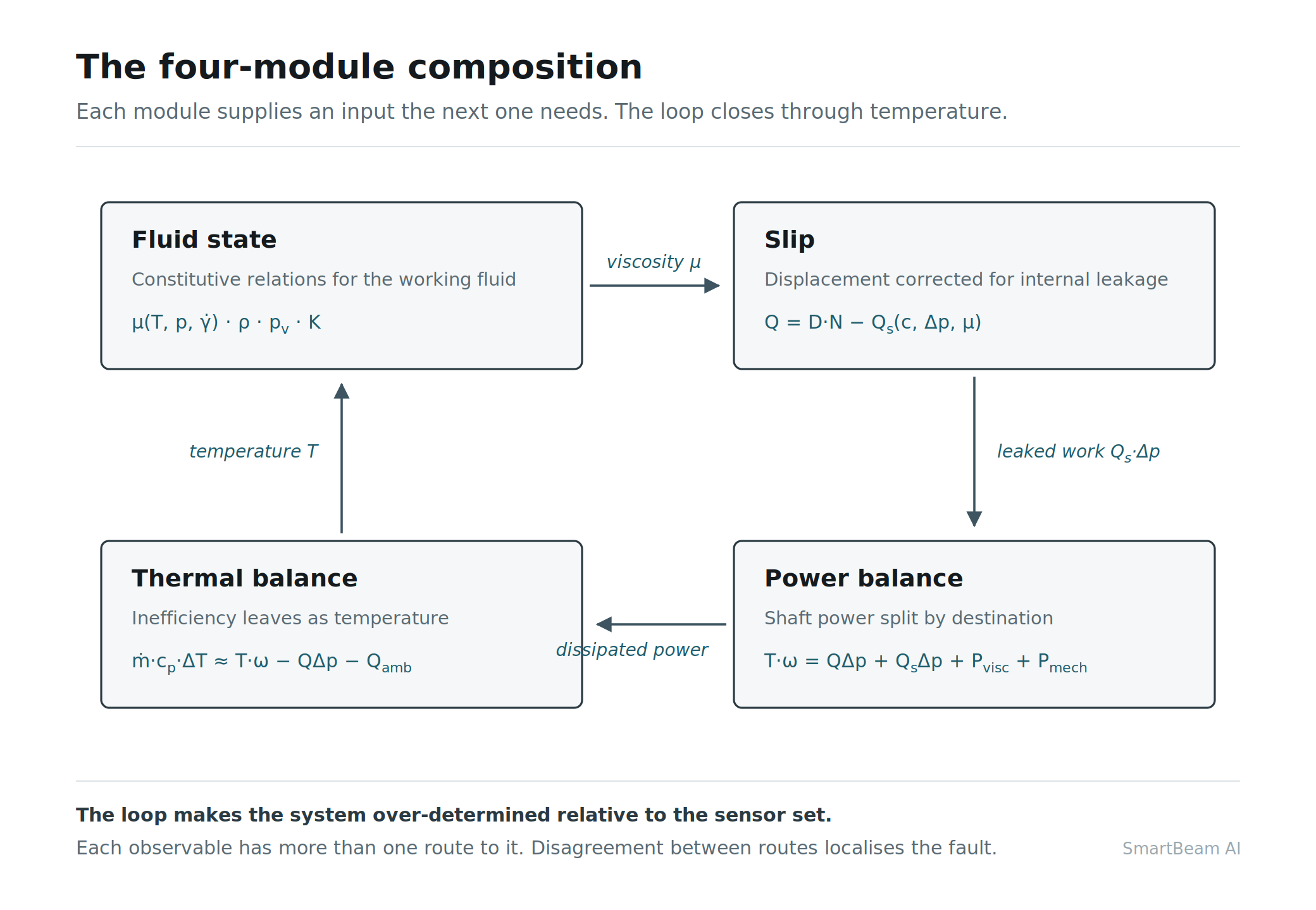
The consequence is that the system becomes over-determined relative to the sensor set. Differential temperature can be predicted from the power-balance route and also measured directly. Delivered flow can be estimated from the slip module and also inferred from the thermal and power routes. Each observable has more than one path to it.
This is the structural property that separates a physics AI engine from a predictor. A single-route model produces an estimate. A multi-route model produces an estimate plus a disagreement between routes, and the disagreement is diagnostic. When the slip route and the thermal route stop agreeing about volumetric efficiency, one of the two underlying assumptions has broken, and which one has broken localises the fault.
4. Virtual sensing and the inverse problem
Two capabilities follow from the composition, and both are worth naming precisely because they are what a customer actually buys.
Virtual sensing. Once the composition is calibrated to a specific machine, it functions as a high-rate soft sensor for quantities nobody has instrumented: chamber pressure through the cycle, flow ripple, pressure spikes at valve events, internal leakage split by path. No intrusive hardware, no process interruption, no meter to foul.
The precedent here is from cardiology. Fractional flow reserve, the reference measurement for whether a coronary narrowing is functionally significant, was historically obtained by threading a pressure wire into the artery. It is now routinely computed instead: blood flow is modelled as a Newtonian fluid governed by the Navier-Stokes equations, applied to CT images, to estimate pressure and flow non-invasively, and the method has demonstrated diagnostic accuracy comparable to the invasive measurement. It has been FDA-cleared since 2014. A physical field that could previously only be reached by inserting hardware into the system is now reached by solving equations against images that were already being taken. That is exactly the trade a virtual flow meter makes on a pump, with the same burden of proof.
Inverse problem solving. The forward problem is easy to state: given clearance, viscosity and speed, predict discharge pressure. The field problem is the reverse. You have discharge pressure, suction pressure, motor current and casing temperature. You want clearance, which nobody can measure without disassembly.
Inverse problems infer unknown parameters, source terms, or initial and boundary conditions from indirect and often noisy measurements, and they are ill-posed: small errors in the data can produce large deviations in the solution. This is why inference of internal condition from surface measurement has historically been the domain of specialists rather than software.
Physics constraints are what make it tractable at scale. Methods of this class can efficiently handle ill-posed inverse problems that are difficult or impossible for conventional numerical treatment, and they tolerate noisy, sparse and multi-fidelity data. Mechanically, the unknown physical parameters become learnable quantities alongside the network weights, and the total loss combines the equation residual, the data misfit and a regularization term on the parameters. The physical law is what removes the ill-posedness: solutions that would fit the data but violate conservation are not in the feasible set.
5. What actually gets trained
Three things sit inside a deployed physics engine, and only one of them is learned from data.
The governing equations are not learned. They are written, and they do not change between installations.
The machine-specific parameters are not learned from a corpus either. Effective clearance, dead volume, valve coefficients and mechanical loss constants are identified per pump by inverse solution against a short characterisation run, by the method in Section 4. This is what removes the white box scaling problem. A new installation does not need an engineer to rewrite the model. It needs a few hours of structured operation to re-identify a dozen numbers.
What is learned is the residual layer, and that is where the leverage is.
The residual formulation
A residual is the disagreement between what the physics predicts and what the sensors report:
r = y_measured − y_predicted(θ, u)
where θ are the identified machine parameters and u the current operating condition. A second family of residuals comes from the over-determination described in Section 3: the gap between two independent physical routes to the same latent state, such as volumetric efficiency estimated through slip and through the thermal balance.
The learned model does not map sensors to a health score. It maps residuals to fault mechanisms. That change of coordinates is what makes the rest work.
The learning problem collapses in size. Physics has already absorbed every deterministic effect: flow rising with speed, slip falling with viscosity, the temperature dependence of both. None of that has to be learned, because none of it survives into the residual. What remains is small, bounded, and close to zero-mean on a healthy machine. A model that has to explain only the leftovers needs a fraction of the data of one that has to explain the entire signal.
Domain shift largely disappears. This matters most on a population of one-off machines. A black box trained at 40 cSt and 12 bar degrades at 4 cSt and 30 bar because the mapping from sensors to health has genuinely changed. A residual is defined after viscosity, pressure and speed have been accounted for, so its distribution under healthy operation is approximately invariant across duty points and fluid regimes. Data collected at one operating point stays informative about another. That is the direct answer to a fleet too small and too heterogeneous to learn from.
Healthy data becomes free and abundant. Every operating hour on every machine produces residuals under known-good conditions, with no labelling effort and no failure required. Label scarcity was the binding constraint on data-driven maintenance for this class of machine. In residual space the constraint is much weaker, because the expensive labels are needed only for the fault classes, and the fault classes live in a low-dimensional space.
The output stays inspectable. A residual carries units and a sign. “Measured differential temperature exceeds prediction by 2.3 K, and the slip and thermal routes to volumetric efficiency disagree by 1.8 points” is a statement an engineer can audit, argue with, and put in a failure report. An anomaly score is not.
Why simulation and hardware compose
Training runs on both, and each supplies what the other cannot.
Simulation contributes labelled fault-mode signatures across severity ladders that no one would induce on a production pump: rotor clearance growth in graded steps, valve seat leakage, timing gear backlash, relief bypass, suction starvation, each crossed with viscosity, differential pressure and speed ranges spanning the operating envelope. It is generated rather than collected, and labelled by construction.
Instrumented hardware contributes what simulation cannot fabricate: real sensor noise, real mounting and foundation effects, real material response, and fault progressions that develop rather than being imposed at a chosen severity.
The two can be mixed because both are expressed as residuals against the same physics engine. They share a coordinate system. Attempts to mix them in raw signal space fail, and the published record on that is unambiguous. A finite element bearing study generated labelled synthetic data across four classes and then tested on hardware: trained on simulation alone, the model reached 61.4 percent on real data3. In both cases the model was learning a mapping in raw signal space, where the simulated and measured distributions differ in every respect the simulation failed to capture, most of which have nothing to do with the fault.
The residual formulation does not abolish that gap. It relocates it. What remains is the error of the physics engine itself, which is one quantity, measurable against instrumented ground truth, and bounded by the procedure in Section 7. An unknown distributional mismatch becomes a number with a confidence interval.
Neither source suffices alone, which is why a serious physics AI programme runs a laboratory. Simulation cannot produce the residual distribution of a real sensor on a real foundation moving a real fluid. Hardware cannot produce forty severity levels across six fault modes and four viscosity regimes inside a development cycle. Training uses both. Validation uses hardware only.
6. Are you measuring slip?
Almost certainly not. Very few positive displacement pumps carry a flow meter, and none carry a clearance gauge. Slip is not measured anywhere in the industry. It is the single most informative variable about the pump’s internal condition, and it is invisible.
Under a physics AI treatment, slip stops being a measurement and becomes an estimated latent state, carrying a confidence interval, produced by inverse solution against the sensors you already have.
Slip is worth the trouble of inferring, for two reasons.
The first is that slip is speed-independent while flow is not. Leakage is driven by differential pressure and viscosity, not by shaft speed, so volumetric efficiency rises with speed purely as an arithmetic consequence. A study of axial piston pumps with a 0.1 mm wear clearance measured volumetric efficiency improving from 67.48 percent to 94.44 percent as speed increased from 500 to 3000 rpm at 20 MPa load, an average gain of 5.39 percentage points per 500 rpm4. The same study found speed to be a larger contributor to volumetric efficiency than load pressure, wear clearance or eccentricity. An efficiency trend that is not speed-corrected and viscosity-corrected is measuring the operator, not the pump.
The second is that slip is where mechanical faults surface as hydraulic symptoms, and this is what makes it the right monitoring variable.
A worked progression: timing gear backlash in a twin screw pump
Twin screw rotors are not supposed to touch. They are synchronised by timing gears, and any play developing in the gear train or bearings allows the rotor profiles to make contact, producing surface damage that degrades the close clearance volumetric efficiency depends on, after which the pump slips more internally and must run faster to hold the same flow.
Trace that through the modules.
| Stage | Physical state | Slip module | Power module | Thermal module | Vibration |
|---|---|---|---|---|---|
| 0 | Nominal clearance | η_v at baseline | Torque matches prediction | ΔT at baseline | Clean gear mesh |
| 1 | Backlash growth, intermittent contact | No change beyond uncertainty | No change | No change | Mesh sidebands appear |
| 2 | Flank scuffing, local clearance growth | Slip rises, and rises with Δp | Slip work term grows | ΔT rises slightly | Sidebands broaden |
| 3 | General clearance growth | η_v down several points | Torque up at constant delivered flow | ΔT clearly elevated | Broadband floor rises |
| 4 | Functional loss | Flow shortfall visible to process | Speed increased to compensate | ΔT high | Late, non-specific |
The table shows two things.
The mechanical module leads at Stage 1 and the hydraulic modules lead at Stage 3. Neither alone gives a continuous picture of the progression. A vibration-only system sees an early gear anomaly and cannot say whether it matters. A performance-only system sees nothing until damage is done. The composition converts two partial views into one trajectory, and a maintenance decision rests on the trajectory rather than the alarm.
The alternative to catching this is expensive. Internal wear increases clearances, slip grows progressively, and the degradation is often invisible to operations because the pump keeps running and simply delivers less per revolution. In many facilities the first indication is a process complaint about low flow or slow transfer times, by which point a substantial fraction of volumetric efficiency is already gone.
The discrimination that only composition can make
Now the harder case, and the one that shows why four modules are needed rather than one.
Relief valve bypass produces the same top-level symptom as clearance wear: delivered flow falls below displacement times speed. A model that monitors volumetric efficiency alone cannot separate them, and the maintenance actions are entirely different.
The modules separate them on three physical grounds.
Pressure dependence. Clearance leakage is continuous and roughly proportional to Δp. Relief bypass is a threshold phenomenon: near zero below the set pressure, steep above it. Fitting the observed flow deficit against Δp distinguishes a slope from a knee.
Viscosity dependence. Clearance leakage scales inversely with viscosity, so it changes measurably when the fluid warms. Relief bypass through a fully open valve is far less viscosity-sensitive. A temperature excursion is therefore a free diagnostic experiment, if the model is watching for it.
Thermal localisation. Slipped fluid dissipates its work inside the pump casing. Bypassed fluid dissipates across the valve. Same energy, different place, and the thermal balance module knows which node it belongs to.
None of these discriminations is available to a model that has learned a mapping from sensors to a health score. All are available to one that carries the equations.
7. Verification, validation and error bounds
This is the stage that separates research from field implementation, and it is the stage most commonly skipped.
Disciplines that put simulation in front of consequential decisions built this framework decades ago, split across two standards answering different questions. One asks how wrong the model is. The other asks how much rigour is enough, given what the answer will be used to decide. A deployed physics engine needs both.
How wrong is it
The ASME standard for verification and validation in computational fluid dynamics and heat transfer quantifies the accuracy of a simulation at a specified validation point, using experimental uncertainty analysis to account for error in both the simulation and the measurement it is compared against. Validation here is an assessment of model error rather than a pass or fail exercise. The difference between simulation and measurement is the centre of an interval that should contain the true model error at a stated confidence, and the width of that interval comes from combining experimental, numerical and parameter uncertainty.
The standard is deliberately narrow, and instructively so. It bounds model error where validation data exists, and treats accuracy away from those points as engineering judgment rather than a computed result. For a pump physics engine that is a design instruction: an operating envelope is not declared, it is validated, point by point, and its edges are wherever the validation points stop.
How much rigour is enough
The second standard is ASME V&V 40, developed with the FDA for computational models that inform medical decisions, and it is the framework SmartBeam assesses its physics engine against. It does not prescribe verification and validation steps. It determines how much rigour those steps require5.
The sequence runs in a specific order. State the question of interest, which includes naming the decision it feeds. State the context of use, meaning the particular role and scope of the model in answering that question. Then establish model risk from two components: model influence, or how far the decision rests on the model rather than on other available evidence, and decision consequence, the severity of an adverse outcome if the model is wrong. Model risk then sets a target credibility level across a set of credibility factors, each with graded levels of rigour, and those goals are fixed before the supporting data are gathered rather than justified afterwards.
It transfers to industrial equipment because the framework was built domain-agnostic. Practitioners applying it outside medical devices substitute their own terms where the clinical vocabulary does not fit, and the rigour demanded of each credibility factor scales with the assessed risk in exactly the same way.
Applied to a pump, one model has several contexts of use, and they do not all demand the same evidence.
| Context of use | Model influence | Decision consequence | Credibility demanded |
|---|---|---|---|
| Trending slip to inform overhaul scope six months out | Low. Bench inspection confirms before work is done | Moderate. Wrong scope, wasted parts | Moderate |
| Extending a scheduled overhaul interval on model evidence | High. The model is the primary evidence | High. Unplanned failure in service | High |
| Prescribing an immediate rate cut or shutdown | High | High. Process upset, possible safety exposure | Highest |
The same engine, the same equations and the same validation data can be sufficiently credible for the first row and not for the third. Collapsing that into a single vendor claim about accuracy is the error the framework exists to prevent.
What a verified engine reports
Translated into pump terms, a verified physics engine does not report that slip is 8.4 percent. It reports 8.4 percent with an interval at a stated confidence, carrying the model error established at validation together with the current measurement uncertainty. It also reports the envelope that interval is good for: this viscosity range, this differential pressure range, this speed range, this fluid class. Outside that envelope it declines to answer.
That has three consequences, each of them a design requirement.
A change is only actionable when it exceeds the validation uncertainty. Reporting a 0.4 percent shift in efficiency when the model error is bounded at 1.1 percent is noise dressed as insight, and it is how condition monitoring systems lose their audience.
The domain of validity must be declared and enforced at runtime. The physics engine must notice when the process has left the envelope it was validated in, and downgrade its own output when it has. Data-driven systems approximate this with out-of-distribution detection, but the boundary they find sits in feature space and carries no physical meaning. An envelope stated in viscosity, pressure and speed is one an operator can read, dispute, and design around.
Prescription requires a higher bar than detection. Telling an operator that something has changed and telling them to stop a pump are different contexts of use carrying different model risk, and under a risk-informed framework they carry different credibility goals. They should not share an error budget.
8. What field implementation looks like
Commissioning a physics AI engine is a calibration exercise, not an installation. The sequence is short, and every stage produces something the plant can hold on to.
| Stage | What happens | Typical duration | What exists at the end |
|---|---|---|---|
| Instrumentation review | Confirm the existing sensor set constrains the parameters to be identified. Add points only where a parameter would otherwise be unobservable | Days, desk-based | A stated list of what the physics engine can and cannot resolve on this machine |
| Characterisation | A structured run across a designed set of duty points, ideally spanning two viscosity states, to inverse-solve effective clearance, dead volume, valve coefficients and mechanical loss constants | Hours of pump operation | A model of tag P-1401A rather than of a pump type |
| Credibility assessment | Set credibility goals per context of use and confirm the evidence meets them, by the method in Section 7 | Once, then on change | A documented statement of what the physics engine may and may not be used to decide |
| Live monitoring | The engine runs forward and tracks residuals against prediction and between independent physical routes | Continuous, from day one | Structured residuals that name a mechanism rather than raise a score |
| Scheduled re-verification | Re-characterisation on the plant’s existing calibration cycle, with triggers on detected envelope violations | Aligned to instrument calibration intervals | A model whose accuracy is a maintained quantity, not an assumption |
Two rows deserve stating plainly, because they are where this differs from what the market offers.
There is no baseline learning period. The physics engine does not need twelve months of history to establish what normal looks like, because normal is computed from the governing equations and the identified parameters. A pump with no failure record and no historian is a valid first day. That is the direct consequence of the residual formulation in Section 5, and it is the question worth putting to any vendor: what does your system know on the morning it is switched on.
Re-verification is a feature of instruments, not a defect of models. Every pressure transmitter and flow meter on site is on a calibration schedule, and nobody calls that a weakness. Physics AI can be put on the same schedule because its accuracy is a measurable quantity. Systems that cannot be re-verified are not systems that stay accurate. They are systems whose drift nobody is measuring.
What the engine needs, and what it does without it
The physics engine needs fluid property data: viscosity against temperature, density, vapour pressure, for the fluid actually being handled. Little of this requires new work. A grade classified under ISO 3448, or any product datasheet quoting kinematic viscosity at two temperatures, is enough to compute viscosity across the operating range by the standard viscosity-temperature relations in ASTM D341, with viscosity index from ISO 2909. The inputs are specifiable before contract rather than discovered during deployment. A system that cannot tell you in advance what it requires is one that will tell you afterwards why it underperformed.
There is a return on that input worth having. When the assumed fluid properties stop matching the observed behaviour of the pump, the physics engine notices, because the mismatch shows up in a residual that clearance and wear cannot explain. Off-specification grade, contamination, water ingress and dilution all present this way. The requirement becomes a diagnostic.
Where the sensor set does not constrain a parameter, the physics engine says so at the instrumentation review rather than estimating it and hoping. Where the process moves outside the validated envelope, it downgrades its own output and states why. The failure mode is a declared abstention, which an operator can act on, rather than a confident wrong answer, which an operator cannot detect.
What a plant can hold the vendor to
Four commitments follow from the architecture rather than from a service level agreement, which is what makes them checkable. Each is traceable to a section above.
Every estimate carries an interval and a declared envelope, so a reported change can be tested against the model’s own error before anyone mobilises.
Every alert names a physical mechanism and a margin in engineering units, which is what a root cause report, a warranty claim and an insurer all require and what a score cannot supply.
Internal condition is inferred from instrumentation the pump already has, without intrusive metering, process interruption or a shutdown to install anything.
The system operates from the first day on a machine with no failure history, on a site with no comparable fleet.
9. Closing
Ask what an industrial AI system scores on a benchmark and you learn something about the benchmark. Benchmarks are drawn from the distribution the model was trained on. Industrial plants are not.
The question worth asking is whether the system can state the conditions under which its answer holds, and refuse when those conditions are not met. That is not a feature bolted onto a model. It follows from building the model out of equations whose domain of applicability is known before anything is deployed.
For positive displacement pumps, where the governing variable is internal, unmeasured and confounded, that is the difference between an analytics product and an instrument.
SmartBeam AI builds physics AI systems for positive displacement pumps. The module composition, residual training and seeded-fault validation described here are implemented in our physics engine, trained on combined simulation and measured data, and validated against instrumented pumps at our PD pump AI Lab, with model credibility assessed under ASME V&V 40.
References
Standards referenced in the text: ASME V&V 20 and V&V 40; ASTM D341; ISO 3448 and ISO 2909.
- Volumetric Efficiency Prediction of External Gear Pumps Using a Leakage Model Based on Dynamic Clearances. Actuators 15(1):56. https://www.mdpi.com/2076-0825/15/1/56 ↩
- Hotvedt, Grimstad and Imsland. On gray-box modeling for virtual flow metering. arXiv:2103.12513. https://arxiv.org/pdf/2103.12513 ↩
- Domain Adaptation from Simulation to Reality: A Transfer Learning Approach for Bearing Fault Diagnosis. Applied Sciences 16(3):1407. https://doi.org/10.3390/app16031407 ↩
- Research on the Influence of Piston Pair Wear on Pump Output Characteristics of Axial Piston Pump Under Multiple Working Conditions. Machines 14(7):753. https://www.mdpi.com/2075-1702/14/7/753 ↩
- An Overview of the ASME V&V 40-2018 Standard. Springer. https://link.springer.com/chapter/10.1007/978-3-032-09180-2_5 ↩